

Produced Water Treatment Cost Optimisation: CAPEX, OPEX and Retrofit Decisions

Contents
Direct answer
Produced water treatment cost optimisation should compare three choices: improve the way the existing plant is operated, retrofit the limiting equipment, or replace part or all of the treatment train. The lowest-cost option is the one that meets the required water quality and capacity with acceptable risk over the remaining field life, not the option with the lowest initial price.
A sound decision includes capital cost, chemical and energy use, maintenance, consumables, waste handling, lost production, off-spec exposure, installation constraints and the value of deferred capital. Diagnose the actual constraint first; otherwise a project may spend money on equipment that does not address the root cause.
Build a complete cost basis
Establish current cost per unit of treated water and the annual cost of the treatment system. Separate fixed and variable costs. Record chemicals, power, gas, filter media, replacement liners, laboratory work, waste and sludge disposal, maintenance labour, vendor support and critical spares.
Add the costs that are often hidden: production curtailment, oil lost with reject water, reinjection impairment, permit risk, emergency mobilisation and repeated troubleshooting. Use normal, peak and late-life water forecasts because a solution that is economic at today’s flow may become a constraint as water cut increases.
Diagnose before choosing the investment
Map where quality or capacity is lost. Use representative samples around each treatment stage and time-align them with flow, pressure, temperature, chemical dose and equipment status. Verify instruments, sample procedures and laboratory methods before using the data to justify capital.
Identify whether the dominant constraint is feed outside the design envelope, inadequate pressure, fine droplets caused by shear, poor gas dispersion, solids loading, worn internals, unreliable chemical delivery, filter fouling or control instability. Several symptoms may share one upstream cause.
When operational optimisation is enough
Optimisation is appropriate when the installed equipment has adequate fundamental capacity and the shortfall results from settings, maintenance, chemistry or controls. Examples include correcting hydrocyclone pressure balance, selecting the active liner count, stabilising flotation level, repairing recirculation, calibrating chemical pumps or improving backwash sequencing.
Low-capital changes should still be tested and documented. Define a baseline, change one variable at a time and prove that gains persist across representative operation. Include the cost of ongoing specialist attention if the new condition is difficult to sustain.
When a retrofit creates the best value
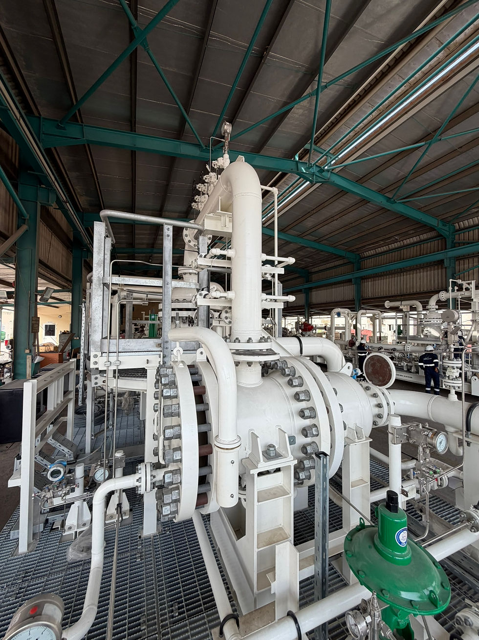
A retrofit is attractive when the pressure vessel, structure and much of the package remain serviceable but a specific component limits performance. Replacement hydrocyclone liners, improved vessel internals, upgraded gas dispersion, sample conditioning, instrumentation or control logic can raise capacity and stability without replacing the whole system.
Brownfield economics must include survey, engineering, isolation, cleaning, transport, offshore or site installation and commissioning. Confirm interfaces and maintenance access. A short installation window or modular change-out can be more valuable than a theoretically cheaper modification that requires a long shutdown.
When replacement is justified
Replacement becomes credible when corrosion or fatigue threatens integrity, the design cannot accommodate future flow, multiple systems are obsolete, utilities are excessive or repeated retrofits would leave a complex and unreliable plant. It may also be the better choice when the disposal route changes and requires a fundamentally different treatment train.
Do not compare a bare equipment price with the full cost of keeping the current plant. Equally, do not assume new equipment eliminates chemical, maintenance or waste costs. Ask for guaranteed performance across the real feed envelope and a transparent list of exclusions.
Compare options with a lifecycle model
Use a common evaluation period, production forecast and discount basis. Model capital expenditure, installation, planned and corrective maintenance, consumables, chemicals, energy, waste, spares and expected downtime. Show uncertainty ranges for water flow, feed quality, service life and installation duration.
Useful outputs include net present cost, cost per treated barrel or cubic metre, payback, production protected and compliance margin. Run sensitivity cases rather than presenting a single precise result. The decision should remain understandable if energy, chemical or disposal prices change.
Evidence and decision process
A practical decision matrix scores each option against water quality, capacity, reliability, safety, schedule, constructability, remaining life and cost. Keep technical gates separate from weighted preferences: an option that cannot meet the outlet requirement should not win because it is inexpensive.
Before publication, add an anonymised lifecycle-cost example and decision matrix. State assumptions clearly and avoid quoting savings without a documented baseline.
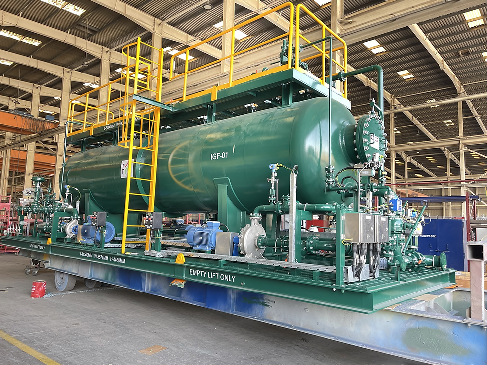
Crescent Engineering can audit existing produced-water systems and compare operational, retrofit and replacement options. Share flow and water-quality data, operating costs, equipment condition and future production profile to compare upgrade options.
References
Crescent Engineering FZE, produced-water optimisation, retrofits and packaged systems.
US DOE National Energy Technology Laboratory, Produced Water Treatment Catalog and Decision Tool.
US Environmental Protection Agency, Oil and Gas Extraction Effluent Guidelines.
US Department of Energy, Management of Produced Water.
Related Crescent articles
Continue exploring this topic:

Comments